Rotational (Cn) symmetry
Learning targets
Using rotational symmetry or Cn boundary specifier
Specify different conditions at different boundaries of the computational domain
This geometry example specifies a isosceles triangular computational domain with Cn boundary identifiers at the left and right legs of the triangle domain and transparent boundaries at the base side of the computational domain. This is a typical situation for propagation mode simulations of multi core optical fibers where the size of the computational domain can be reduced by a factor of N when symmetry considerations about the geometry and the source are taken into account.
The resulting geometry and mesh correspond to the following figure:
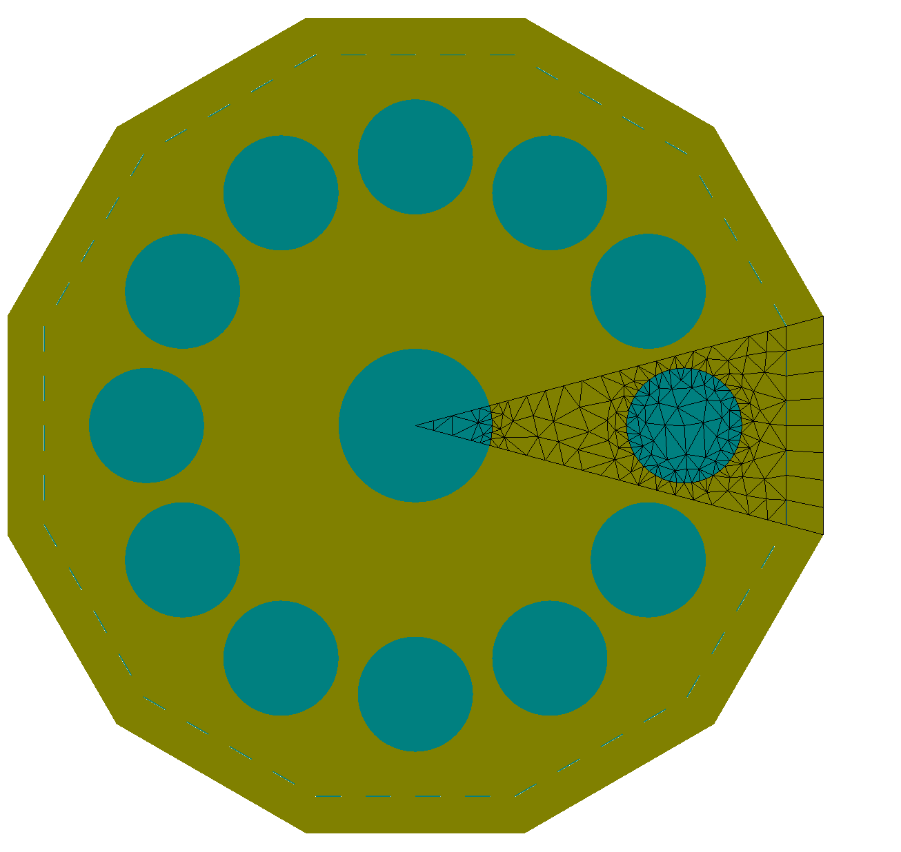
The geometry is automatically unfolded by JCMview. Only shown mesh elements are present in the grid.
.jcm Input File
layout.jcm [ASCII]
 1Layout2D {
 2  MeshOptions {
 3    MaximumSideLength = 1
 4  }
 5  Objects {
 6    Triangle {
 7      DomainId = 1
 8      Priority = ComputationalDomain
 9      Port = Point1
10      Width = 10
11      AngleAlpha = 30
12      AngleBeta = 75
13      RotationAngle = -15
14      Boundary {
15        Class = Cn
16        Number = [1 3]
17      }
18      Boundary {
19        Class = Transparent
20        BoundaryId = 2
21      }
22    }
23    Circle {
24      DomainId = 2
25      GlobalPosition = [0 0]
26      Radius = 2
27      MeshOptions {
28        BoundaryMeshConstraint = .2
29      }
30    }
31    Circle {
32      DomainId = 2
33      GlobalPosition = [7 0]
34      Radius = 1.5
35      MeshOptions {
36        BoundaryMeshConstraint = .2
37      }
38    }
39
40  }
41}
42