Analysis and Optimization Toolkit

The following section contains the documentation for using JCMsuite’s analysis and optimization toolkit from within Python.

The toolkit is provided by the server JCMoptimizer. All Python commands to interact with the JCMoptimizer are described in the Python Command Reference. The available drivers for performing various numerical studies are described in the Driver Reference. The driver reference also includes various simple Python code examples. A tutorial example for a parameter optimization can be found here.

The toolkit enables, for example, the efficient parameter optimization or sensitivity analysis of expensive black-box functions. Typically, the evaluation of these objective functions involves the finite-element solution of a photonic structure. However, the toolkit can be used in conjuction with any function that can be evaluated with Python.

A numerical study consists of retriving parameter values from the server at which the objective function is to be evaluated. The result of the evaluation is sent back to the server. After the study is finished, the results (e.g. the optimal parameter values) can be retrieved from the server. During the run of the study, the progress is vizualized on a dashboard.

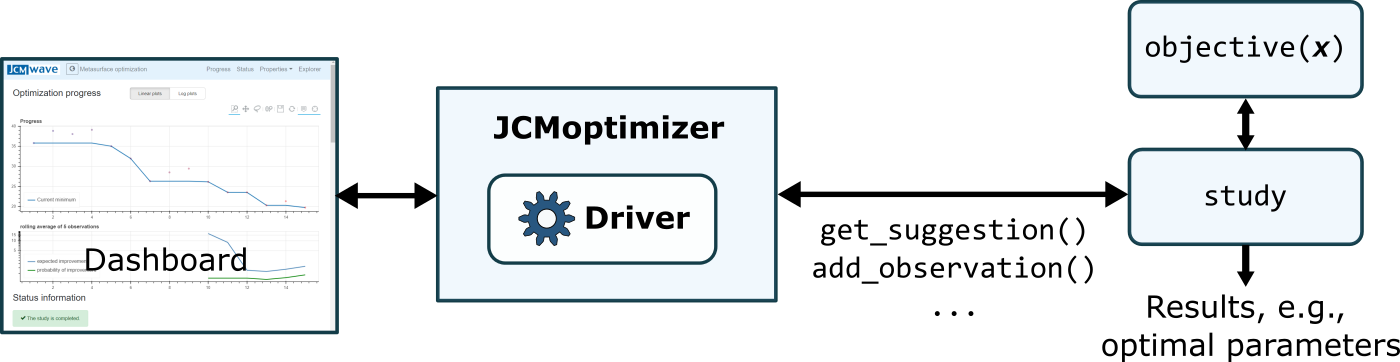
Schematic of the interplay between Python and JCMoptimizer.

Basic usage

Here a code with some basic principles on how to perform an optimization study:

import numpy as np
import jcmwave

# Definition of the search domain
domain = [
    {'name': 'x1', 'type': 'continuous', 'domain': (-1.5,1.5)},
    {'name': 'x2', 'type': 'continuous', 'domain': (-1.5,1.5)}
]

# Creation of the optimization study object. This will automatically
# open a browser window with a dashboard showing the optimization progress.
study = jcmwave.optimizer.create_study(domain=domain, name="Example")
study.set_parameters(max_iter=90)

# Definition of the objective function that will be minimized
def objective(x1,x2):
  observation = study.new_observation()
  observation.add(10*2
              + (x1**2-10*np.cos(2*np.pi*x1))
              + (x2**2-10*np.cos(2*np.pi*x2))
          )
  return observation

# set the objective function and run the optimziation loop
study.set_objective(objective)
study.run()

Extended functionality

This is an example demonstrating some extended functionality:

import os
import numpy as np
import threading
import tempfile
import matplotlib.pyplot as plt
import jcmwave

# Definition of the search domain with continuous, discrete and fixed parameters
domain = [
    {'name': 'x1', 'type': 'continuous', 'domain': (-1.5,1.5)},
    {'name': 'x2', 'type': 'continuous', 'domain': (-1.5,1.5)},
    {'name': 'x3', 'type': 'discrete', 'domain': [-1,0,1]},
    {'name': 'radius', 'type': 'fixed', 'domain': 2},
]

# Definition of a constraint on the search domain
constraints = [
    {'name': 'circle', 'constraint': 'sqrt(x1^2 + x2^2) - radius'}
]

# Creation of the optimization study with a predefined study_id and
# path save_dir where the information of optimization runs are stored
# under the name study_id+'.jcmo'.
save_dir = tempfile.gettempdir()
study = jcmwave.optimizer.create_study(domain=domain, constraints=constraints,
                         name="Extended example - phase 1", study_id="extended_example",
                         save_dir=save_dir)

# Definition of the objective function. In order to speed up the minimization process
# derivative information is provided
def objective(x1,x2,x3,**kwargs):
  observation = study.new_observation()
  observation.add(10*2
              + (x1**2-10*np.cos(2*np.pi*x1))
              + (x2**2-10*np.cos(2*np.pi*x2))
              + 5*x3**2
          )
  observation.add(derivative='x1', value= 2*x1 + 20*np.pi*np.sin(2*np.pi*x1))
  observation.add(derivative='x2', value= 2*x2 + 20*np.pi*np.sin(2*np.pi*x2))
  observation.add(derivative='x3', value= 10*x3)
  return observation

# Sometimes some objective function values are known, e. g., from
# previous calculations. These can be added manually to speed up
# the optimization.
obs = objective(0.7,0.6,0.0)
study.add_observation(obs,sample=dict(x1=0.7,x2=0.6,x3=0.0))

# Run 2 objective function evaluations in parallel
# Stop when the probability of improvement is lower than 1e-5
# Do the first hyperparameter optimization only after 30 observations
study.set_parameters(num_parallel=2, min_PoI=1e-5, optimization_step_min=30)

# Sometimes the evaluation of the objective function fails. Since the
# corresponding observation cannot be added, the suggestion has to be removed
# from the study
suggestion = study.get_suggestion()
study.clear_suggestion(suggestion.id, 'Evaluation failed')

# The objective evaluations are performed in parallel threads.
# If an evaluation fails, the corresponding suggestion is cleared.
def acquire(suggestion):
     try: observation = objective(**suggestion.kwargs)
     except: study.clear_suggestion(suggestion.id, 'Evaluation failed')
     else: study.add_observation(observation, suggestion.id)

# Run the minimization
while (not study.is_done()):
     suggestion = study.get_suggestion()
     t = threading.Thread(target=acquire, args=(suggestion,))
     t.start()

# Now the found minimum is converged via gradient descendent (L-BFGS-B)
info = study.info()
sample = info['min_params']
study2 = jcmwave.optimizer.create_study(study_id=study.id, name="Extended example - phase 2",
                             save_dir=save_dir, driver='L_BFGS_B_Optimization')

# The single minimizer (num_initial=1) stops if the stepsize (eps) is below 1e-9
# By setting max_num_minimizers to 1, one prevents that the minimizer restarts at a
# different position after convergence
study2.set_parameters(num_initial=1, eps=1e-9, max_num_minimizers=1, jac=True,
                      initial_samples=[sample])
study2.set_objective(objective)
study2.run()

# Plot the optimization progress
info = study2.info()
data = study2.get_data_table()
plt.title('Minimum found at ({x1:0.3e}, {x2:0.3e}, {x3:0.0f})'.format(**info['min_params']))
plt.plot(data['iteration'],data['cummin'])
plt.xlabel('iterations')
plt.yscale('log')
plt.ylabel('minimal objective value')
plt.grid(True)
plt.show()

#delete results file
os.remove(os.path.join(save_dir,'extended_example.jcmo'))