Loops¶

In this section we show how to exploit loops (for, while) within Matlab code snippets to define complicated geometries or project setups in a few number of script lines.

Loops within an embedded Matlab code block (cf. previous section Matlab Code Snippets) may extend over several blocks:

<?
for centerX = [0 : 1 : 9]
  keys.center = [centerX 0.0]
?>

Circle {
  Radius = 0.5
  GlobalPosition = %(center)e
  ...
}

<?
end 
?>

Here, a for-loop starts in line 2 within the first Matlab block. This loop is closed in line 13 after a .jcm code block (lines 6-10). Line 3 dynamically sets the value for key center, which serves as circle’s center in line 8. This way, we have defined ten circles, equally spaced in $x$ -direction.

To see how this works in practice, we want to compute the light scattering off multiple rods aligned on a hexagonal lattice. Figure “Multiple rod geometry” shows the setup.

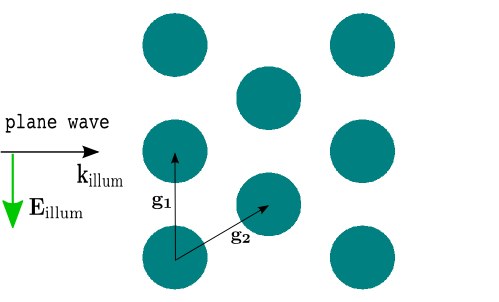
_images/phc_geometry.png — Multiple rod geometry¶

$\pvec{g}_1$ and $\pvec{g}_2$ are called grid vectors. For a hexagonal alignment we have

$\begin{eqnarray*} \pvec{g}_1 = a\cdot\left( \begin{array}{c} 0.0 \\ 1.0 \end{array} \right), \; \pvec{g}_2 = a\cdot \left( \begin{array}{c} \sin(60^\circ) \\ \cos(60^\circ) \end{array} \right), \end{eqnarray*}$

with a lattice parameter $a$ , which is passed as a further parameter in the driver script:

%% set problem parameter
keys.radius = 0.3; 
keys.n_air = 1.0;
keys.n_glass = 1.52;
keys.lambda_0 = 0.550; % in um 
keys.polarization = 45; % in degree
keys.a = 1.0;
keys.n_rods = [3 3];
  
%% run the project
results = jcmwave_solve('mie2D.jcmp', keys);

%% get scattering cross section
scattering_cross_section = ...
  results{2}.ElectromagneticFieldEnergyFlux{1};
fprintf('\nscattering cross section: %.8g\n', ...
        real(scattering_cross_section)); 

%% plot exported cartesian grid within matlab:
cfb = results{3};
amplitude = cfb.field{1};
intensity = sum(conj(amplitude).*amplitude, 3);
pcolor(cfb.X, cfb.Y, intensity); 
shading interp; view(0, 90); axis equal;

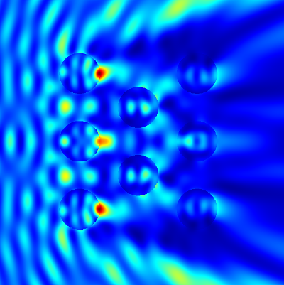
In line 8 we set the number of rods in $x$ - and $y$ - direction. Figure “Intensity” shows the computed intensity of the electric field.

_images/phc_intensity.png — Intensity¶

Pseudo-color intensity plot as produced by the driver `run.m`.

For this problem you again find a driver run_geo.m which only runs the mesh generation:

%% set geometry parameters
keys.radius = 0.3;
keys.a = 1.0;
keys.n_rods = [3 3];

%% generate mesh file only
jcmwave_geo('.', keys);

%% open grid.jcm in JCMview
jcmwave_view('grid.jcm');

You can use this script to “play” with the geometry parameters and to watch how the geometry is updated.

In the following we want to discuss the updated layout file:

<?
  % compute grid vectors for hexagonal grid
  gv1 = [0.0 keys.a];  
  gv2 = [sind(60) cosd(60)]*keys.a;

  % compute computational domain enclosing all scatterer
  maxX = (keys.n_rods(1)-1)*gv2(1);
  maxY = (keys.n_rods(2)-1)*gv1(2);
    
  keys.computational_domain_X = maxX+2*keys.radius+2;
  keys.computational_domain_Y = maxY+2*keys.radius+2;     
?>


Layout2D {
  UnitOfLength = 1e-6

  MeshOptions {
    MaximumSideLength = 0.1
    CurvilinearDegree = 2
  }

  Objects {
    # Computational domain
    Parallelogram {
      DomainId = 1
      Width = %(computational_domain_X)e
      Height = %(computational_domain_Y)e
  
      # set transparent boundary conditions
      Boundary{
        Class = Transparent
      }
    }
  
<?
  center_array = [maxX/2 maxY/2];
  for iX=0 : keys.n_rods(1)-1
    col_start  = [iX*gv2(1) mod(iX, 2)*gv2(2)];
    for iY=0 : keys.n_rods(2)-1-mod(iX, 2);
      keys.center = col_start+iY*gv1-center_array;
     
      
?>
    # Scatterer (rod)
    Circle {
      DomainId = 2
      Radius = %(radius)e
      GlobalPosition = %(center)e
    }
  
<?
    end
   end
?>
  }
}


 

The first Matlab block computes the grid vectors $\pvec{g}_1,$ $\pvec{g}_2$ (lines 2-4), and adapts the computational domain size to enclose all rods (lines 6-11). There, maxX and maxY are the dimensions of the array of rods in $x$ and $y$ .

The Matlab block from lines 34-42 defines two for loops over the number of rods in $x$ and $y$ . Line 39 sets the center of the current rod, which is used in line 46 in the enclosed .jcm block (center_array is used to shift the center of the array of rods to the origin). The for loops are closed in the last Matlab block (lines 51-54).