Graded Index Fiber
In this tutorial project the fundamental propagation modes of a
graded index fiber are computed.
In a graded index fiber, the refractive index of the core is not
constant in space but depending on radial distance from the
optical axis of the fiber.
The functional dependence of refractive index in the core region
is defined as a python expression in the file materials.jcm.
In this case the permittivity  depends
on radial distance
depends
on radial distance  as follows:
 with core radius
  ,
,
 ,
,
 , and
, and
 .
.
Compare the syntax in the file materials.jcm:
materials.jcm [ASCII]
 1Material {
 2  Name = "Cladding"
 3  DomainId = 1
 4  RelPermeability = 1.0
 5  RelPermittivity = 2.0736
 6}
 7
 8Material {
 9  Name = "Core"
10  DomainId = 2
11  RelPermeability = 1.0
12  RelPermittivity {
13    Python {
14      Expression = "this_radius = power(power(X[0], 2) + power(X[1], 2), 0.5);
15                    delta = (power(n1, 2) - power(n2, 2))/(2*power(n1, 2));
16                    value = power(n1, 2)*(1 - 2*delta*power((this_radius/radius), exponent_g));
17                    value = value*eye(3, 3)"
18      Parameter {
19        Name = "n1"
20        VectorValue = 1.45
21      }
22      Parameter {
23        Name = "n2"
24        VectorValue = 1.44
25      }
26      Parameter {
27        Name = "exponent_g"
28        VectorValue = 1.9
29      }
30      Parameter {
31        Name = "radius"
32        VectorValue = 9.5e-6
33      }
34    }
35  }
36}
Definition of the geometry:
layout.jcm [ASCII]
 1Layout2D {
 2  UnitOfLength = 1.0e-6
 3  MeshOptions {
 4    MaximumSideLength = 15
 5  }
 6  Objects {
 7    Circle {
 8      Name = "Cladding"
 9      DomainId = 1
10      Priority = -1
11      Radius = 50.0
12      RefineAll = 2
13      Boundary {
14        BoundaryId = 1
15        Class = Domain
16      }
17    }
18    Circle {
19      Name = "Core"
20      DomainId = 2
21      Priority = 1
22      Radius = 9.5
23      MeshOptions {
24        CurvilinearDegree = 2
25        MaximumSideLength = 4
26      }
27    }
28  }
29}
The tangential electric field components of the fields are expected to be decayed to zero at the boundaries of the computational domain:
boundary_conditions.jcm [ASCII]
1BoundaryCondition {
2  BoundaryId = 1
3  Electromagnetic = TangentialElectric
4}
Accuracy settings and post process definitions (here, also the spatially dependent permittivity field is exported for visualization/cross-checking purposes):
project.jcmp [ASCII]
 1Project {
 2  InfoLevel = 3
 3  Electromagnetics {
 4    TimeHarmonic {
 5      PropagatingMode {
 6        Lambda0 = 1.55e-06
 7        FieldComponents = ElectricXYZ
 8        SelectionCriterion {
 9          NearGuess {
10            Guess = 1.45
11            NumberEigenvalues = 2
12          }
13        }
14        Accuracy {
15          FiniteElementDegree = 3
16          Precision = 1e-4
17          Refinement {
18            MaxNumberSteps = 1
19          }
20        }
21      }
22    }
23  }
24}
25
26PostProcess {
27  ExportFields {
28    FieldBagPath = "project_results/fieldbag.jcm"
29    OutputFileName = "project_results/permittivity_field.jcm"
30    OutputQuantity = RelPermittivity
31    Cartesian {
32      NGridPointsX = 150
33      NGridPointsY = 150
34    }
35  }
36}
37PostProcess {
38  ExportFields {
39    FieldBagPath = "project_results/fieldbag.jcm"
40    OutputFileName = "project_results/e_field_cartesian.jcm"
41    OutputQuantity = ElectricFieldStrength
42    Cartesian {
43      NGridPointsX = 150
44      NGridPointsY = 150
45    }
46  }
47}
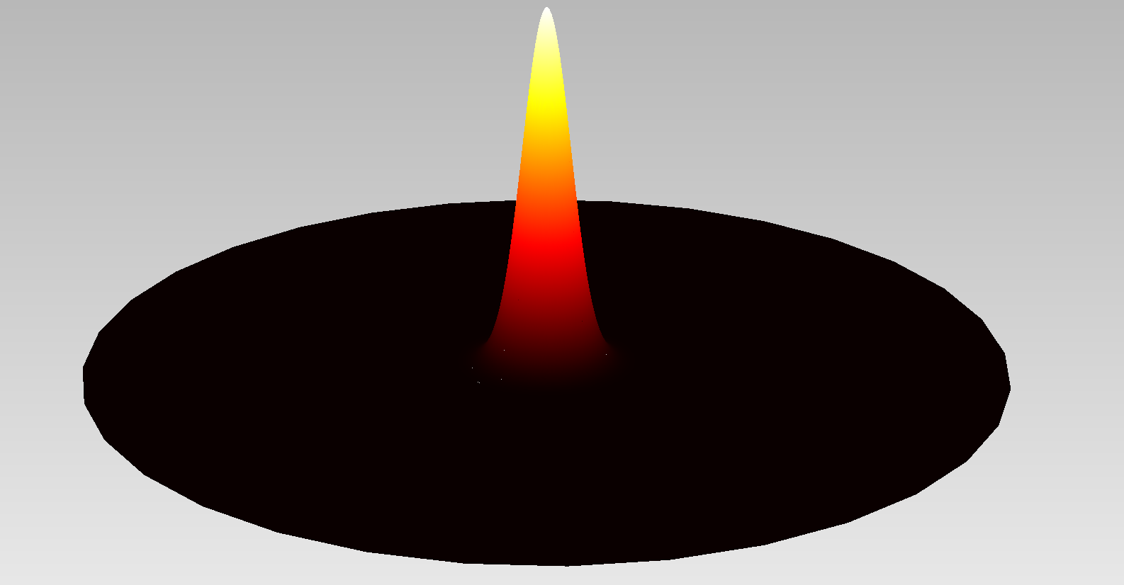
A visualization of the field intensity distribution of a computed mode is shown in the figure below.