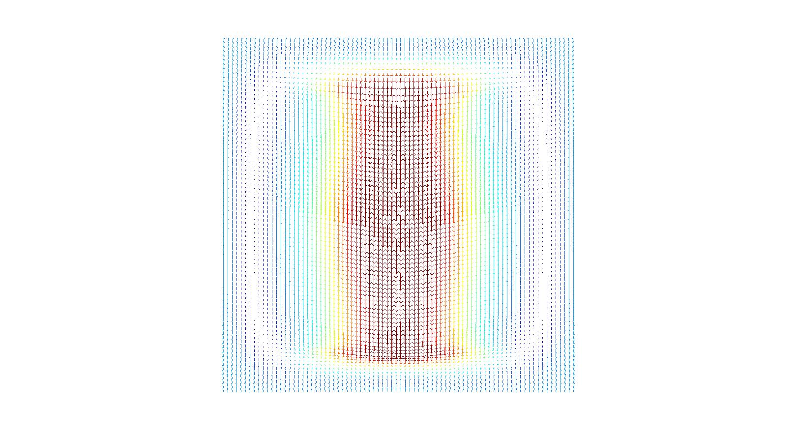
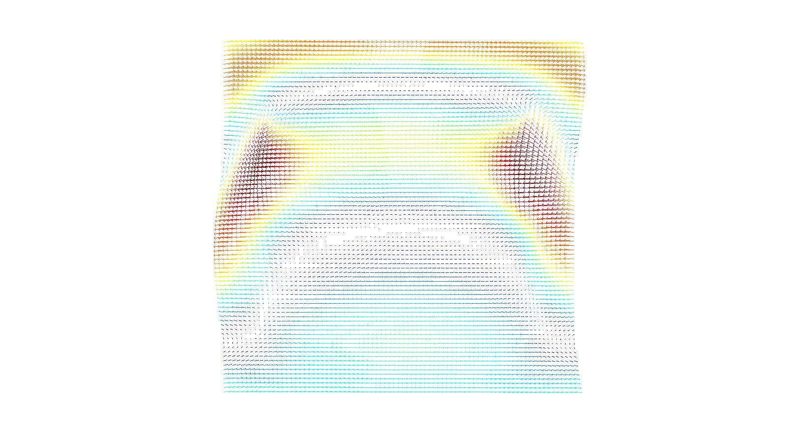
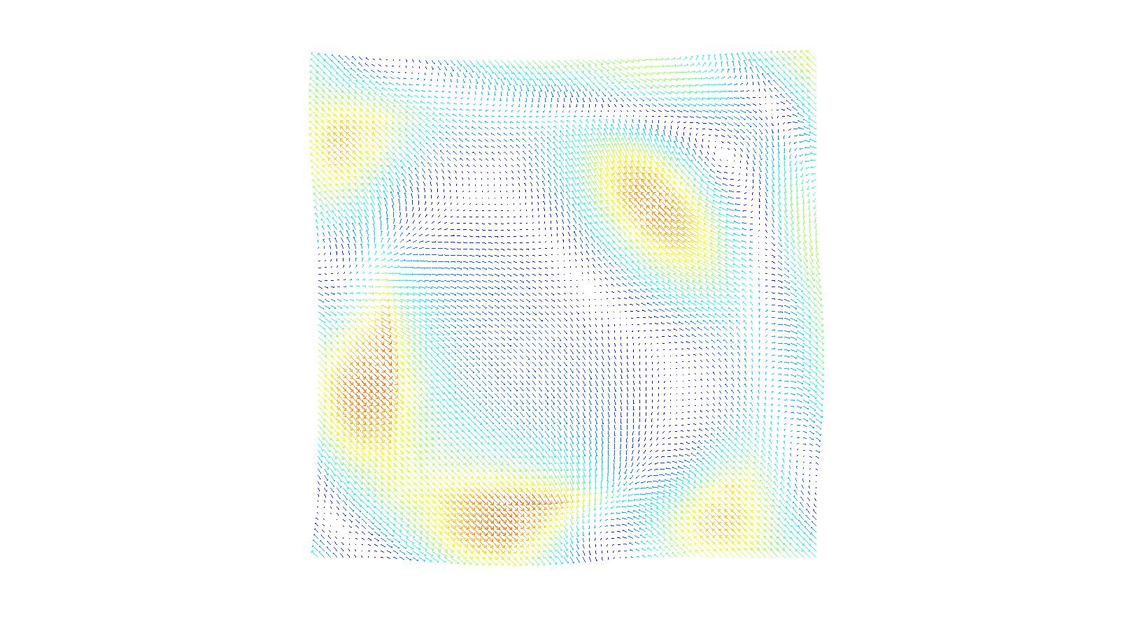
Isolated Contact Hole
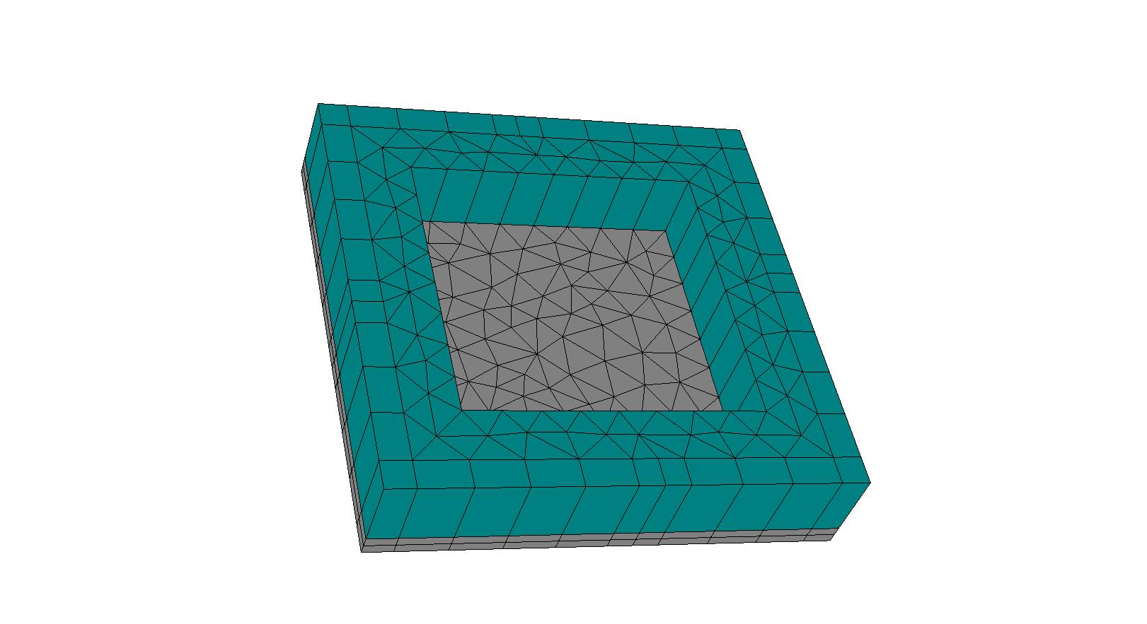
This tutorial example demonstrates simulation of an isolated contact hole, as depicted below:
The geometrical setup defined in the layout.jcm file is:
 1Layout3D {
 2  UnitOfLength = 1e-09
 3
 4  MeshOptions {
 5    MaximumSideLength = 50
 6  }
 7  BoundaryConditions {
 8    Boundary {
 9      Direction = Vertical
10      Class = Transparent
11    }
12  }
13  Extrusion {
14    Objects {
15      Parallelogram {
16        Name = "ContactHole"
17        DomainId = 2
18        Width = 280
19        Height = 280
20      }
21
22      Polygon {
23        Name = "ComputationalDomain"
24        DomainId = 1
25        Priority = -1
26        Boundary {
27          Class = Transparent
28        }
29        ConvexHull {
30          Parent = "ContactHole"
31          Offset = 50
32        }
33      }
34    }
35
36    MultiLayer {
37      Layer {
38      Bottom {
39        GlobalZ=-50
40      }
41      Thickness = 50
42      DomainIdMapping = [1 3 2 3]
43    }
44    Layer {
45      Thickness = 72
46      DomainIdMapping = [1 2 2 1]
47    }
48    Layer {
49      Thickness = 50
50      DomainIdMapping = [1 1 2 1]
51    }
52
53  }
54}
55}
56
The given parallelogram defines the hole on the mask with side length 280nm. Since this pattern is modelled as isolated, it is surrounded by the absorbing mask material in lateral direction. In JCMsuite this is conveniently set up by defining a ConvexHull around a geometrical primitive. This automatically sets up a convex hull with minimum distance Offset to the enclosed pattern. For the ConvexHull the DomainId and Priority and Boundary can be defined as usual.
Since the mask pattern is isolated, any number of incident plane waves with same frequency and different incident direction can be defined as sources:
  1SourceBag {
  2  Source {
  3    ElectricFieldStrength {
  4      PlaneWave {
  5        Lambda0 = 193e-9
  6        Incidence = FromBelow
  7        Sigma = [0 0]
  8        SP = [1 0]
  9      }
 10    }
 11  }
 12}
 13
 14SourceBag {
 15  Source {
 16    ElectricFieldStrength {
 17      PlaneWave {
 18        Lambda0 = 193e-9
 19        Incidence = FromBelow
 20        Sigma = [0 0]
 21        SP = [0 1]
 22      }
 23    }
 24  }
 25}
 26
 27SourceBag {
 28  Source {
 29    ElectricFieldStrength {
 30      PlaneWave {
 31        Lambda0 = 193e-9
 32        Incidence = FromBelow
 33        Sigma = [0.5 0]
 34        SP = [1 0]
 35      }
 36    }
 37  }
 38}
 39
 40SourceBag {
 41  Source {
 42    ElectricFieldStrength {
 43      PlaneWave {
 44        Lambda0 = 193e-9
 45        Incidence = FromBelow
 46        Sigma = [0.5 0]
 47        SP = [0 1]
 48      }
 49    }
 50  }
 51}
 52
 53SourceBag {
 54  Source {
 55    ElectricFieldStrength {
 56      PlaneWave {
 57        Lambda0 = 193e-9
 58        Incidence = FromBelow
 59        Sigma = [0 0.5]
 60        SP = [1 0]
 61      }
 62    }
 63  }
 64}
 65
 66SourceBag {
 67  Source {
 68    ElectricFieldStrength {
 69      PlaneWave {
 70        Lambda0 = 193e-9
 71        Incidence = FromBelow
 72        Sigma = [0 0.5]
 73        SP = [0 1]
 74      }
 75    }
 76  }
 77}
 78
 79SourceBag {
 80  Source {
 81    ElectricFieldStrength {
 82      PlaneWave {
 83        Lambda0 = 193e-9
 84        Incidence = FromBelow
 85        Sigma = [0.5 0.5]
 86        SP = [1 0]
 87      }
 88    }
 89  }
 90}
 91
 92SourceBag {
 93  Source {
 94    ElectricFieldStrength {
 95      PlaneWave {
 96        Lambda0 = 193e-9
 97        Incidence = FromBelow
 98        Sigma = [0.5 0.5]
 99        SP = [0 1]
100      }
101    }
102  }
103}
The sigma coordinates in the pupil plane are used to define different incident directions. At the bottom a number of plots of the transmitted fields are shown. The post process FourierTransform is defined similarly to a periodic setup. In the isolated case, however a discrete representation of the continuous FourierTransform of the mask’s far field is computed. The continuous Fourier transform is thereby sampled on a Cartesian mesh in k-space.