High Power Diode Laser
In this tutorial project we study the effect of heating on the mode profile of a realistic diode laser, namely thermal lensing. A change in temperature leads to a change of the refractive index of a material. This of course effects the shape and propagation constant of waveguide modes. Usually heating increases the refractive index, which leads to a lateral squeezing of modes.
The following figure shows the cross section of the super large optical waveguide laser we analyze:
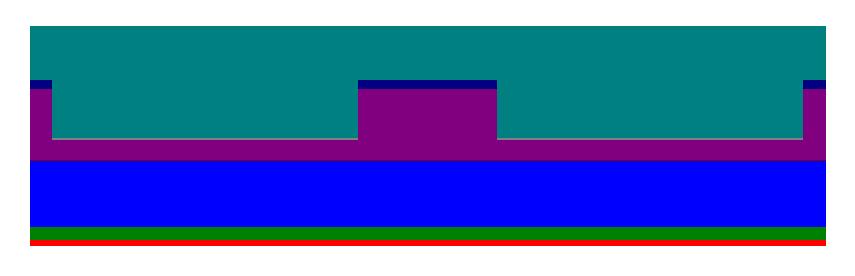
The diode laser consists of a pn-junction. The lateral waveguide for the lasing modes is formed by two trenches, etched into the structure. The cross section is set up from a number of parallelograms in the layout file.
Heat conduction project
In order to study the effect of temperature on the propagating modes, we first have to determine the temperature distribution within the device. The corresponding project files are located in a separate sub folder heat. The length scale of the temperature distribution are of course much larger than the optical profile. Also the global mounting of the device, heat sinks, etc. have to respected. Therefore we increase the size of the layout for the temperature simulation:
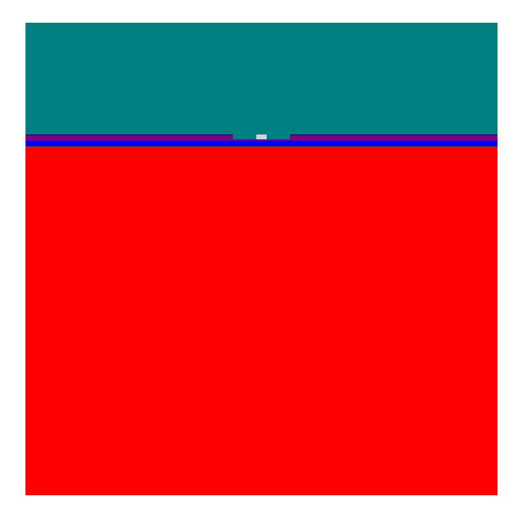
The layout of the heat problem and the propagating mode problem in the base folder only differ by the size of the computational domain, which crops all other defined parallelograms. Further, in the heat layout, we have one additional parallelogram which is used to define the location of the thermal source between the trenches:
Parallelogram {
  Name               = "Heater"
  DomainId           = 1000
  Priority           = 3
  ...
}
In the source file the following heat source is defined:
SourceBag {
  Source {
    DomainId = 1000
    ThermalSourceDensity = 4e13
  }
  Source {
    BoundaryId=1
    Temperature  = 293
  }
  Source {
    BoundaryId=2
    Temperature  = 293
    Emissivity   = 1.0
  }
}
which assigns a spatially uniform thermal source to the parallelogram with DomainId=1000 and specifies the temperature sources for the boundaries.
The boundary conditions for the thermal simulation are:
BoundaryCondition {
  BoundaryId   = 1
  Thermal      = Fixed
}

BoundaryCondition {
  BoundaryId   = 2
  Thermal      = Radiating
}
The Fixed boundary condition sets the temperature profile to the given Temperature and models a heat sink. The Radiating boundary condition is the open boundary condition for thermal simulation and models heat emission into an infinite ambient. The corresponding temperatures for the boundaries are defined in the source file.
The project for heat simulation is:
Project {
  InfoLevel = 3
  HeatConduction {
    Static {
      FiniteElementDegree = 2
      Accuracy {
        Refinement {
          MaxNumberSteps = 2
          PreRefinements = 0
        }
      }
    }
  }
}
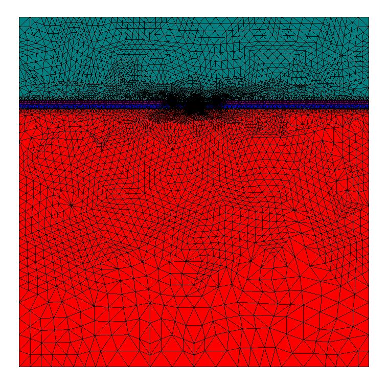
It has similar solving options as electromagnetic simulations, however the project branch is HeatConduction and Static. The resulting temperature distribution with the given thermal source is shown in the following:
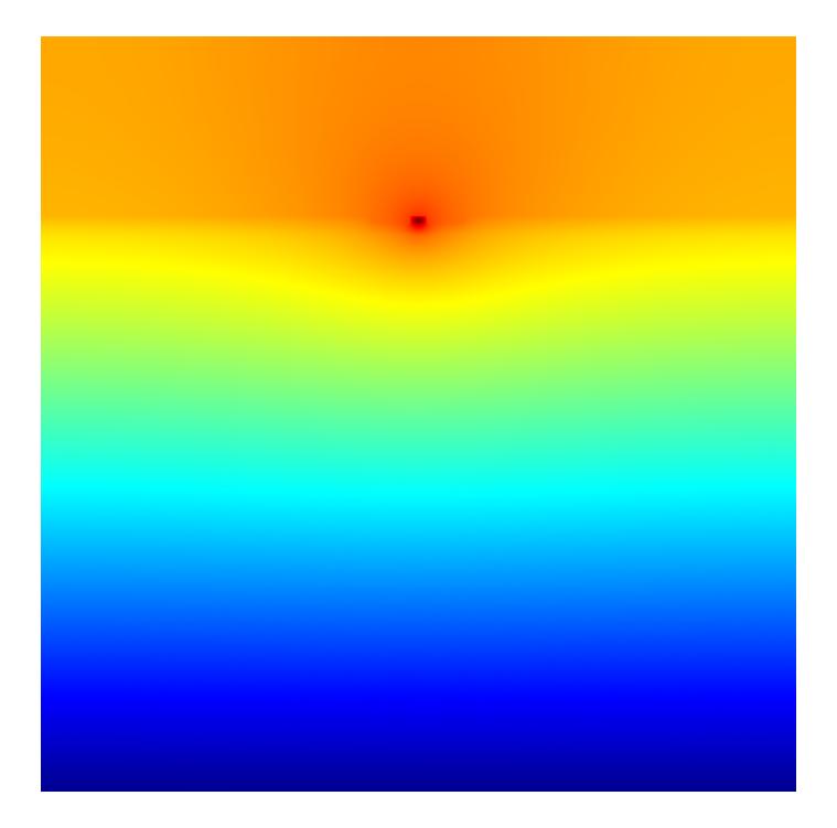
Also for heat simulations adaptive mesh refinement is available and the self-adaptive grid refinement, clearly refines the grid where the temperature field solution shows most pronounced features
Coupling of thermal effects to optical simulation
The physical influence of rising temperature on an optical simulation is modelled by a change in the refractive index. JCMsuite provides a thermo optical correction to the permittivity which is defined in the materials file :
Material {
  ...
  RelPermittivity {
    Constant = (12.1, 0.0006)
    ThermoOpticalCorrection {
      C=0.00173925271362718
      T0=293
    }
  }
  ...
}
The RelPermittivity is described by a fixed Constant value plus a linear correction term, with coefficient C. For a temperature of T0=293 the correction is zero. The temperature profile computed previously can now be used to continuously correct the refractive index according to above linear dependence. The temperature field is selected in the sources file :
SourceBag {
  Source {
    Temperature {
      FieldBag {
        FileName="heat/project_results/fieldbag.jcm"
      }
    }
  }
}
We chose the FieldBag which was the result of the temperature simulation. The computed fundamental mode is depicted in the following:

The project definition uses standard settings as in our basic propagating mode example.
Thermal lensing
In order to quantify the effect of thermal lensing, we defined a reference project in the Reference sub folder. The only difference to the temperature dependent mode project is the sources file definition:
SourceBag {

  Source {
    Temperature = 293
  }
}
which sets a constant Temperature = 293 on the whole computational domain. For comparison of the width of the mode, we export the computed eigenmodes on a slice in the active zone in a post process. This is defined in the project file :
PostProcess {
  ExportFields {
    FieldBagPath = "project_results/fieldbag.jcm"
    OutputFileName = "project_results/mode_slice.jcm"
    Format = JCM-ASCII
    Cartesian {
      NGridPointsX = 1000
      GridPointsY=[1e-9]
    }
  }
}
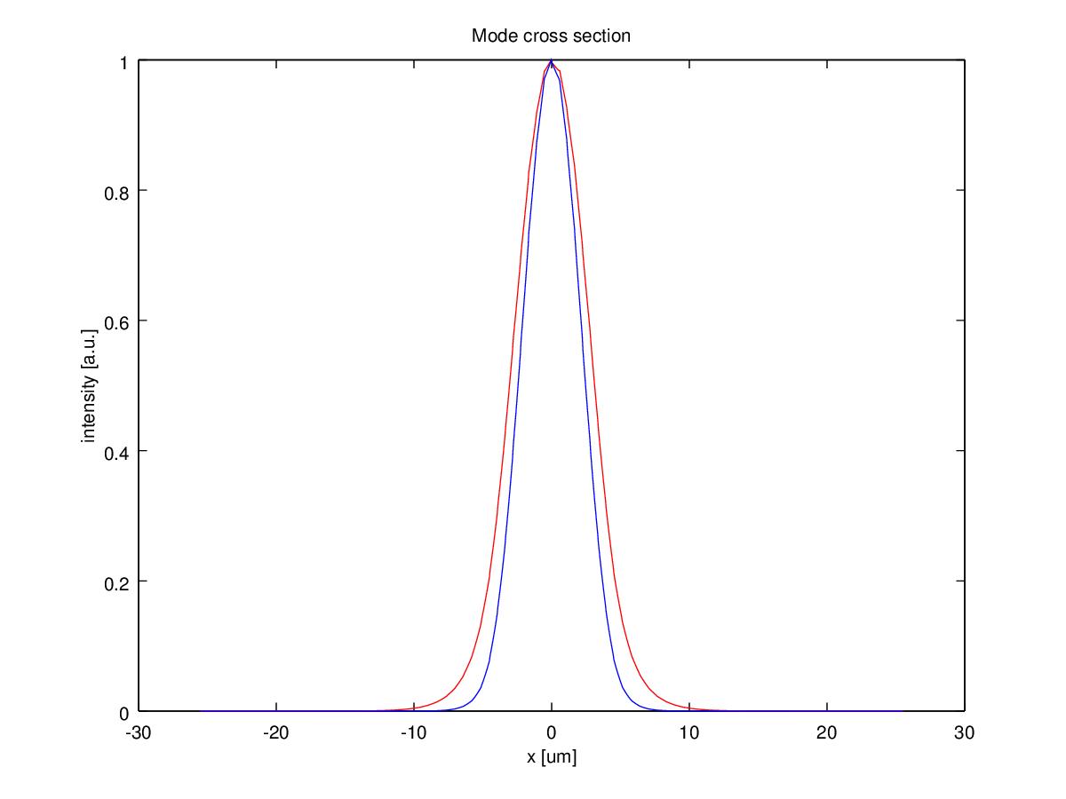
For visualization in Matlab® or Octave we provided a small script plot_slice.m which can be used to plot the exported cross section of a mode:
>> plot_slice('Reference/project_results/mode_slice.jcm',4,'r')
Above command plots the intensity of the 4th mode of the specified file in color 'r'. Plotting the reference mode (red) and the temperature dependent mode (blue) into the same plot, we can clearly observe the thermal lensing effect: