Pinhole
This example computes light propagation of incident plane waves (at oblique angle of incidence) through an isolated pinhole:
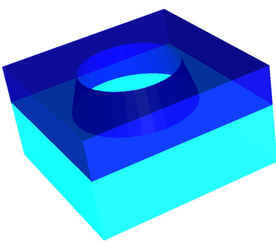
Pinhole geometry
The following figure shows a vector plot of the computed near field.
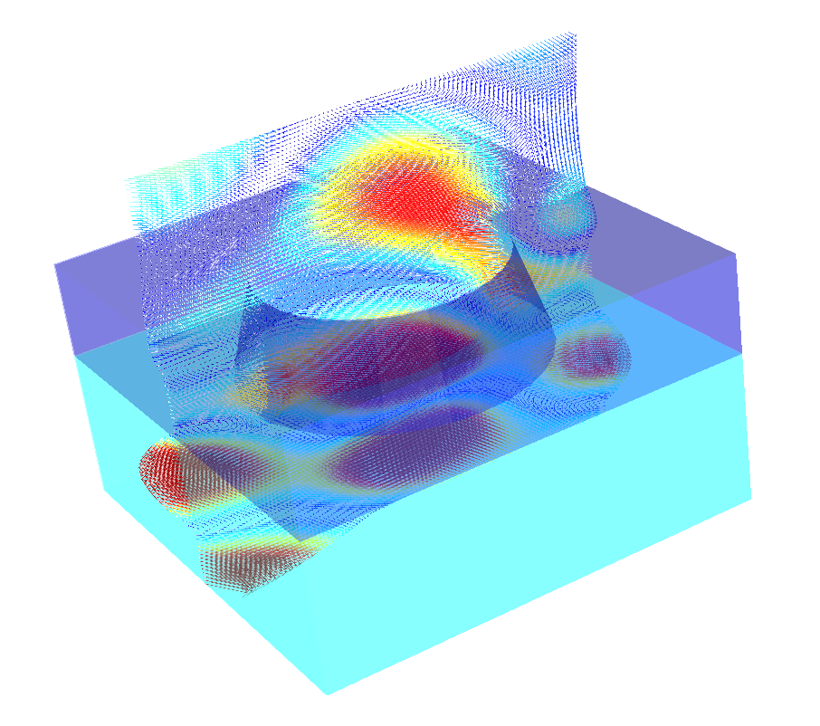
Vector plot of the near field.
Note
Since the geometry of this setup is cylindrical symmetric you can also use (at higher numerical efficiency) the solver for 3D problems with rotational symmetry for this example. This is shown in section Exploiting Rotational Symmetry.
The geometry has transparent boundary conditions in the traversal  -directions. Therefore, the Fourier transform of the scattered field is no longer discrete as for periodic problems. Hence, the Fourier transform post-process actually approximates a continuous function in
  -space.
In an experiment the far field is typically collected by an optical setup forming an image. The post-process OpticalImaging allows to describe a general optical imaging system. We demonstrate this for a simple  -magnification tool without aberrations.
PostProcess {
  OpticalImaging {
  InputFileName = "project_results/transmitted_fourier_transform.jcm"
  OutputFileName = "project_results/image_fourier_transform.jcm"
  OpticalSystem {
    SpotMagnification = 2.0
  }
}
The output file image_fourier_transform.jcm" contains the Fourier transform of the field, after passing the optical system.
You can use a Cartesian export post-process to compute the coherent image.
The following figure shows the image in different  -slices (image planes displaced along -direction), for
  -polarized illumination.
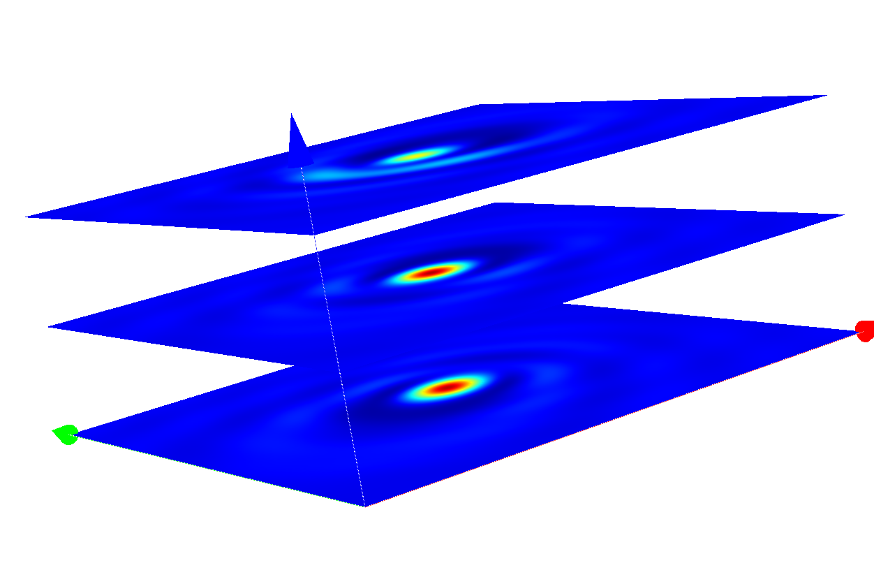
Coherent images of the pinhole after passing the optical system.