Isolated Scatterer
The chiral response of optical scatterers may be computed in JCMsuite using the formalism of the optical chirality and
the built-in Chiral Quantities. It has been shown that the time-harmonic optical chirality density obeys a local
continuity equation [1]. This enables the analysis of chiral behaviour analogous to a standard extinction experiment
studying electromagnetic energy.
In the case of energy, the extinction is composed of scattering and loss [2]. The corresponding chiral quantities
are the extinction  and scattering
  of optical chirality as well as the chirality conversion in volumes
  and on interfaces
  . This yields the conservation law
where integration is performed on the exterior surface  and in the volume
  and on the surface
  of the scatterer.
These quantities are named within JCMsuite as shown in the following table. Further details may be found here.
|
 |
|
 |
|
 |
|
 |
As an example, we compute the chiral response of the scatterer depicted below:
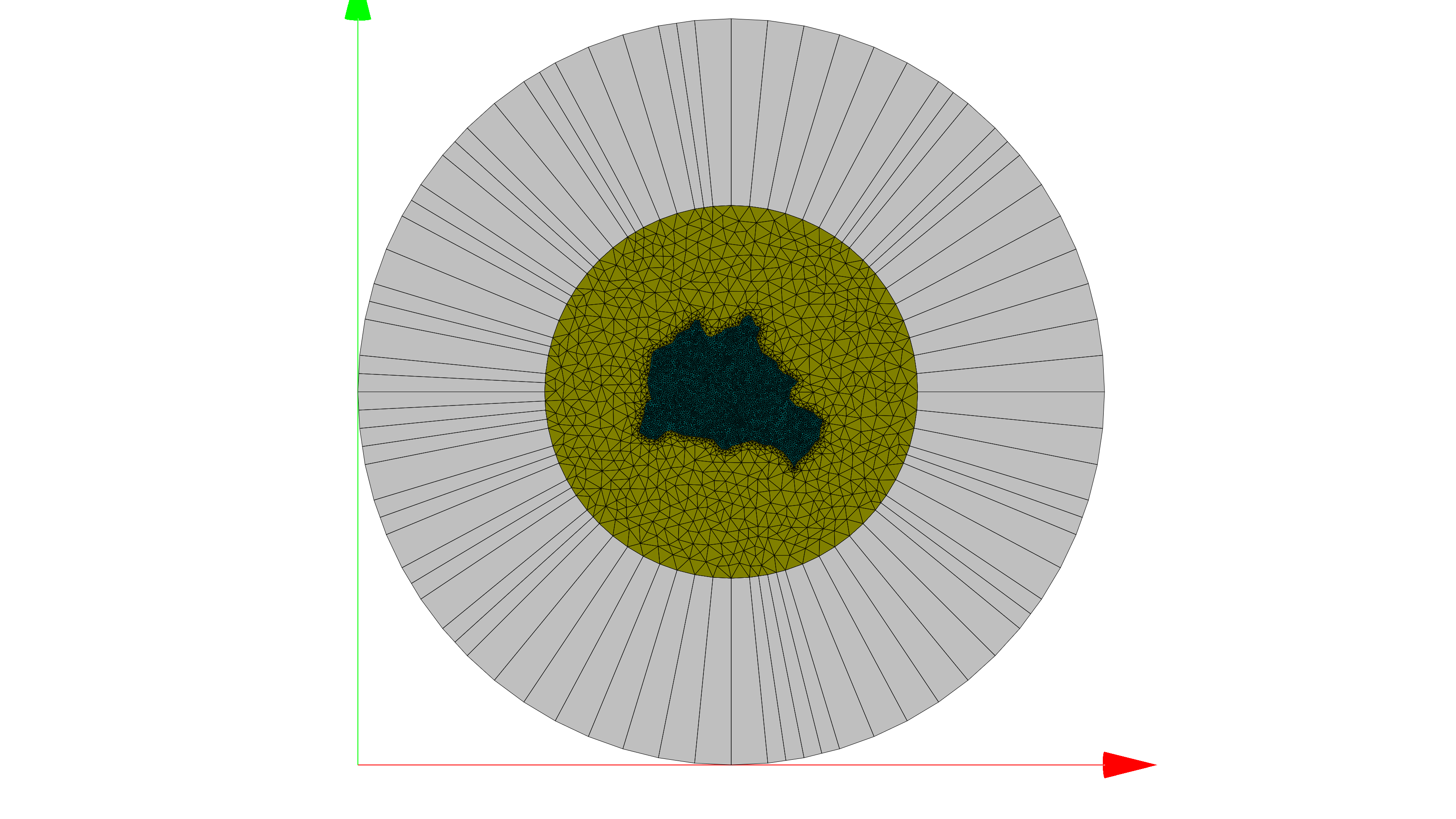
Its diameter is of the order of one wavelength and its permittivity is fixed as  .
In the following, we will vary the permeability
.
In the following, we will vary the permeability  of the scatterer and observe the predicted dual symmetry [3] for a constant ratio
  of the scatterer and its environment.
The surrounding material is air with
of the scatterer and its environment.
The surrounding material is air with  .
.
Since the scatterer is lossless and isotropic, there will be no conversion within its volume. Please refer to the example of a quarter-wave plate for further information on volume conversion.
Here, the required quantities are computed as FluxIntegration of the ElectromagneticChiralityFlux as described above. As shown in the plot below, the conversion tends to zero for materials approaching the dual symmetry as expected.
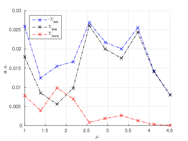
Variation of the permeability of the scatterer for a fixed permittivity  . The scatterer is dual for
  yielding zero chirality conversion.
All chiral densities are accessible as similar quantities within JCMsuite. For example, we show the electric part of the
enhanced near-field optical chirality density in the figure below . This is obtained as a PostProcess, namely ExportFields with the OutputQuantity ElectricChiralityDensity.
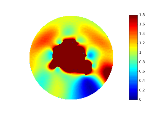
Near-field enhancement of the optical chirality density  for a dual scatterer with .
Bibliography
| [1] | Philipp Gutsche, Lisa V. Poulikakos, Martin Hammerschmidt, Sven Burger, and Frank Schmidt. Time-harmonic optical chirality in inhomogeneous space. In SPIE OPTO, Vol.9756m pages 97560X. International Society for Optics and Photonics, 2016. |
| [2] | Craig F. Bohren and Donald R. Huffman. Absorption and Scattering of Light by Small Particles. John Wiley & Sons, 1940. |
| [3] | Ivan Fernandez-Corbaton. Helicity and duality symmetry in light matter interactions: Theory and applications. PhD thesis, Macquarie University, Department of Physics and Astronomy, 2014. |