Static¶

Type:	section
Appearance:	simple

This section defines a project to compute the stationary deformation of a body, when exposed to prescribed loading conditions such as external forces or initial stresses. The major aim is to compute the arising internal stresses.

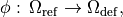
In the following, $\VField{u}$ denotes the displacement field. The original body filling the reference domain $\Omega_{\reff}$ is deformed to a body $\Omega_{\mathrm{def}}.$ The deformed body is related to the reference body by the deformation mapping $\phi=\VField{u}+id$ ,

$\begin{eqnarray*} \phi:\, \Omega_{\reff} \rightarrow \Omega_{\mathrm{def}}, \end{eqnarray*}$

and one defines the component-wise deformation gradient $\nabla \VField{\phi}:$

$\begin{eqnarray*} \nabla \VField{\phi} & = & \left [ \begin{array}{ccc} \partial_x \phi_x & \partial_y \phi_x & \partial_z \phi_x \\ \partial_x \phi_y & \partial_y \phi_y & \partial_z \phi_y \\ \partial_x \phi_z & \partial_y \phi_z & \partial_z \phi_z \\ \end{array} \right ] \equiv \partial_j \phi_i \end{eqnarray*}$

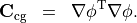
A non-constant deformation field gives rise to a local change of the metric (compared to the reference body) which is given by the Cauchy-Green deformation tensor,

$\begin{eqnarray*} \TField{C}_{\mathrm{cg}} & = & \nabla \phi^{\mathrm{T}} \nabla \phi. \end{eqnarray*}$

The derivation from the original Euclidean metric is called strain and is quantified by the Green-Lagrangian strain tensor

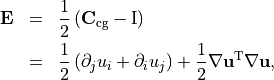
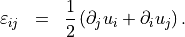
$\begin{eqnarray*} \TField{E} & = & \frac{1}{2} \left( \TField{C}_{\mathrm{cg}}-\mathrm{I} \right) \\ { } & = & \frac{1}{2} \left(\partial_j u_i + \partial_i u_j \right ) + \frac{1}{2} \nabla \VField{u}^{\mathrm{T}} \nabla \VField{u}, \end{eqnarray*}$

which is expressed in terms of the displacement field $\VField{u}$ . Within the linear theory the second, quadratic term is neglected and the so gained linear strain is denoted by $\TField{\varepsilon}$ ,

$\begin{eqnarray*} \TField{\varepsilon}_{ij} & = & \frac{1}{2} \left(\partial_j u_i + \partial_i u_j \right ). \end{eqnarray*}$

Warning

A linear model is used. It is only valid for sufficiently small displacements.

Within the linear theory the constitutive relation between the stress and the (linear strain) reads as

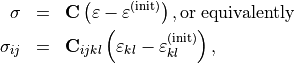
$\begin{eqnarray*} \TField{\sigma} & = & \TField{C} \left( \TField{\varepsilon}-\TField{\varepsilon}^{(\init)} \right), \mbox{or}\;{\mbox{equivalently}} \\ \TField{\sigma}_{ij} & = & \TField{C}_{ijkl} \left( \TField{\varepsilon}_{kl}-\TField{\varepsilon}^{(\init)}_{kl} \right), \end{eqnarray*}$

where $C$ is the stiffness tensor and $\varepsilon^{(\init)}$ is the prescribed initial strain.

The equations governing linear elasticity follow from the minimum principle for the elastic energy:

$\begin{eqnarray*} \int_{\Omega} \TField{\varepsilon} : \TField{\sigma} - \VField{u} \VField{F} = \int_{\Omega} \varepsilon_{ij} C_{ijkl} \left ( \varepsilon_{kl}-\varepsilon_{kl}^{(\init)} \right ) -u_i F_i & \rightarrow & \min \end{eqnarray*}$

This condition is supplemented by boundary conditions, c.f., boundary condition section ContinuumMechanics.

Plane strain problems

Prismatic structures, such as an optical fiber, with a $z$ -dimension much larger than the cross-section diameter are treated by the plane strain assumption: It is assumed that the strain tensor is independent of the $z$ -coordinate and that all entries of the strain tensor involving a $z$ -direction are zero, that is, 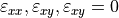$\varepsilon_{xx}, \varepsilon_{xy}, \varepsilon_{xy} = 0$ . In this case a two dimensional grid file has to be passed to JCMsolve.

Implicitly defined quantities

The table below lists field quantities which are implicitly defined within the solution fieldbag. This way they can be used by subsequent post-processes.

Quantity	Expression	JCM Tag
Strain	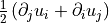$\frac{1}{2} \left( \partial_j u_i + \partial_i u_j \right )$	Strain
Stress	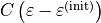$C\left(\varepsilon- \varepsilon^{(\init)} \right)$	Stress

Bibliography

[1]	Braess D., Finite elements: theory, fast solvers, and applications in solid mechanics, Cambridge University Press, 2001.

[2]	Okamoto K., Fundamentals of Optical Waveguides, Academic Press, 2006.